Comparison of machine learning methods in email spam detection
11 February 2018 • 8 min read • Classification, Spam • comments
Unsolicited bulk emails, also known as Spam, make up for approximately 60% of the global email traffic. Despite the fact that technology has advanced in the field of Spam detection since the first unsolicited bulk email was sent in 1978 spamming remains a time consuming and expensive problem.
This report compares the performance of three machine learning techniques for spam detection including Random Forest (RF), k-Nearest Neighbours (kNN) and Support Vector Machines (SVM).
Introduction
Despite the rising popularity of instant messaging technologies in recent years, email continues to be the dominant medium for digital communications for both consumer and business use. Following industry estimations (Symantec Corporation, 2016, pp 31 1), approximately 200 billion emails were sent each day in 2015. On average, business users sent and received around 42 emails per day. Given those facts, it is no wonder that email is still the weapon of choice for cybercriminals who want to target the broadest possible audience electronically.
According to Nucleus Research (Nucleus Research, 2007 2), spam costs US businesses an average of $712 per employee every year due to diminished productivity, lost customers, spent bandwidth and increasing the cost of maintenance.
Estimates (Statista, 2017 3) are that slightly less than 60 percent of the incoming business email traffic is unsolicited bulk email (known as spam) which was the lowest level since 2003. However, even though the global percentage of spam/ non-spam ratio is decreasing, the competition between spammers and spam filtering techniques continuous. It is fair to say that the problem is not going away, and the need for reliable anti-spam filters remains high.
The idea of automatically classifying spam and non-spam emails by applying machine learning methods has been pretty popular in academia and has been a topic of interest for many researchers.
Knowledge engineering and machine learning are the two main approaches scientists have been applied to overcome the spam-filtering problem. The first solution focuses on creating a knowledge-based system in which pre-defined rules dictate if an incoming message is legitimate or not. The primary disadvantage of this method is that those rules need to be maintained and updated continuously by the user or a 3rd party like for example a software vendor.
The machine learning approach, in contrast, does not require pre-defined rules, but instead messages which have been successfully pre-classified. Those messages make the training dataset which is being used to fit the learning algorithm to the model. One could say the algorithm defers the classification rules from the test data.
This study compares three algorithms which are suitable for classification problems. In particular, we included the following methods:
- Random Forest
- k-Nearest Neighbours
- Support Vector Machines with Linear Kernel
For the experiment, we use Hewlett Packard’s Spambase dataset which is publicly available and downloadable from the UCI Machine Learning Repository.
Methods
The following part provides a brief introduction to the three methods used for the experiment and compares general advantages and disadvantages.
Random Forest
Tin Kam Ho first introduced the general method of random decision forests at AT&T Bell Labs in 1995 (Tin Kam Ho, 1995 4). The thought is, that
If one tree is good, then many trees (a forest) should be better.
Stephen Marsland, 2014, p. 275 5
The algorithm deducts the classification label for new documents from a set of decision trees where for each tree, a sample is selected from the training data, and a decision tree is created by choosing a random subset of all features (hence “Random”). The algorithm is suitable for complex classification tasks in small datasets (Breiman, 2001 6). By averaging multiple trees, random-forest-based models have a significantly lower risk of overfitting and include less variance compared to decision trees. The major drawback is performance as a large number of trees may make the method slow for real-time prediction.
k-Nearest Neighbours
The k-nearest neighbour (kNN) classifier is a straightforward method and works well for simple recognition problems. It is considered as an example-based classifier because the training data is used for comparison and not for explicit category representation. In literature, the term lazy-learner is also often related to kNN.
When a new document needs to be categorised, kNN tries to find the k nearest neighbours (most similar documents) in the training dataset. Given that, enough neighbours are found and have been categorised, kNN uses their profile to assign the new document to the same category. This comparison is a real-time process, and therefore the main drawback of this approach is that the kNN algorithm must compute the distance and sort all the training data for each prediction, which can be slow if given a large training dataset (James, Witten, Hastie, & Tibshirani, 2013, pp. 39–42 7).
Support Vector Machines
The original Support Vector Machines algorithm was designed by Vladimir N. Vapnik and Alexey Ya. Chervonenkis in 1963 (Vapnik & Chervonenkis, 1964 8). SVM has its foundation in the broad concept of decision planes which define the decision boundaries. Decision planes separate distinct objects by finding the optimal hyperplane with the maximum margin between two separate classes. SVM provides high accuracy on small and clean datasets but tends to perform less efficient on noisier datasets with overlapping classes (James et al., 2013, pp. 349–359 7).
Procedure
The following part describes the experiment procedure including exploratory data analysis, model fitting, evaluation and prediction.
Exploratory Data Analysis
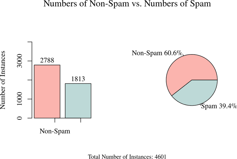
The Spambase dataset was composed by Mark Hopkins, Erik Reeber, George Forman, and Jaap Suermondt at Hewlett-Packard Labs. The set includes a total of 4601 observations from Mr Foreman’s personal email account, 2788 messages are classified as Non-Spam and 1813 were effectively Spam (cf. figure 1).
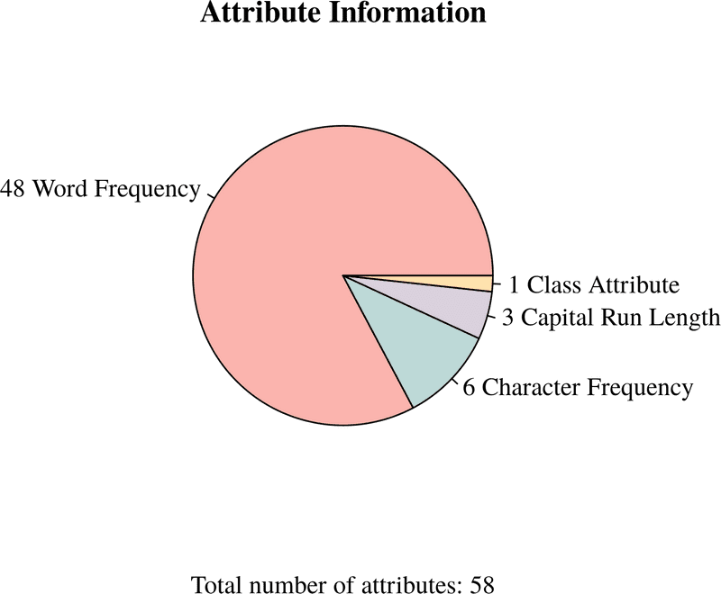
58 different attributes were computed of which 57 are continuous and one is a nominal class label. Typically, documents are represented as vectors of word frequencies. The dataset includes measurements for 6 character frequencies and 48 different word frequencies such as “Internet”, “George” (Mr Foreman’s first name), “Credit”. Furthermore, three data points were collected which represent the average, the maximum and the total length of character sequences in uppercase (cf. figure 2).
Feature Selection
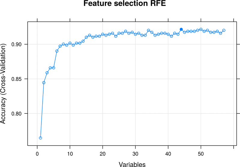
A widely used algorithm for automatic feature selection is Recursive Feature Elimination or RFE. It is based on the idea of repeatedly constructing models and select either the worst- or best-performing feature. RFE than removes the feature from the stack and repeats the process with the remaining features in the set.
Figure 3 illustrates RFE applied with a Random Forest algorithm to the Spambase dataset. All 57 attributes have been selected in the example, although the plot shows that selecting just 44 attributes provide similar accuracy.
Classification tree
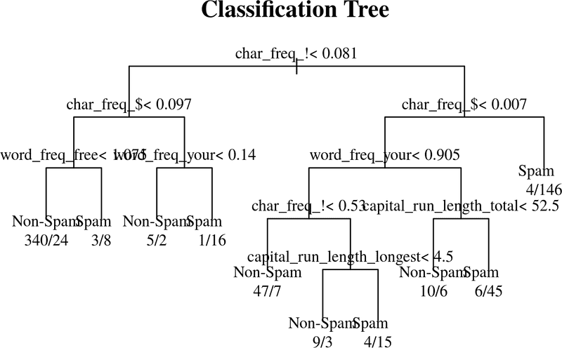
Another handy technique in data mining is recursive partitioning. This method helps to visualise the decision rules for a particular prediction. Figure 4 shows an example of a classification tree on the Spambase dataset.
Training
After we have completed our initial data exploration analysis, we now prepare the data and train our models using the three describe methods. The data preparation involves the following steps:
- Set human readable column names on the data frame
- Replace the class data with descriptive label where zero represents “Non-Spam” and a one marks a record as “Spam”
- Cast the class column to data type factor as the caret package complains if labels are 0 or 1
- Take samples from 1000 and split those into test and training sets randomly with a training/ test ratio of 70%
Prediction and evaluation
Finally, after we have completed the training step for all three models let us have a look how they compare to each other regarding performance. We compare the performance of all three approaches by evaluating the most commonly used indicators: spam precision (SP), spam recall (SR) and accuracy (A). All three indicators originate from the confusion matrix of each model (cf. figure 5).
- Spam precision is the percentage of correct results divided by the number of all returned results
- Spam recall is the percentage of all Spam emails which are correctly classified as Spam
- The accuracy is the percentage of all emails that are correctly categorised
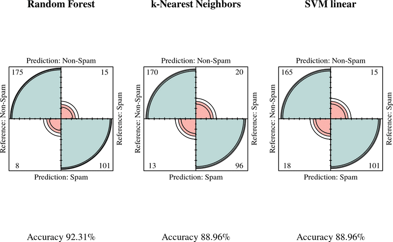
The table below summarises the performance result of all three machine learning methods. We determine from the results that k-Nearest Neighbours (kNN) and Support Vector Machine (SVM) perform similar weak regarding accuracy and Random Forest (RF) outperforms both. We see that RF and SVM have the same relatively high percentage of spam recall while kNN performs significantly worse in that category. Finally, we learn that RF has the highest percentage of spam precision and SVM almost 10 points less than RF.
| Algorithm | Spam Precision (SP) | Spam Recall (SR) | Accuracy (A) |
|---|---|---|---|
| Random Forest | 92.66 | 87.07 | 92.31 |
| k-Nearest Neighbours | 88.07 | 82.76 | 88.96 |
| SVM Linear | 94.87 | 87.07 | 88.96 |
Conclusion
By the looks of the result, one could say that using the random forest approach is the gold way, although we need to keep in mind that we have not fine tuned any of those models at all! Therefore due to its design Random Forest performs relatively well “out-of-the-box” compared to k-Nearest Neighbours and Support Vector Machine.
References
-
Symantec Corporation. (2016). Internet Security Threat Report (Vol. 21).
↩ -
Nucleus Research. (2007). Spam costing US Businesses $712 Per Employee.
↩ -
Statista. (2017). Global spam email traffic share 2014-2017.
↩ -
Tin Kam Ho. (1995). Random decision forests. Proceedings of 3rd International Conference on Document Analysis and Recognition, 1, 278–282.
↩ -
Stephen Marsland. (2014). Machine Learning: An Algorithmic Perspective (2nd ed.). Chapman; Hall/CRC.
↩ -
Breiman, L. (2001). Random Forests. Machine Learning, 45 (1), 5–32.
↩ -
James, G., Witten, D., Hastie, T., & Tibshirani, R. (2013). An Introduction to Statistical Learning.
↩ -
Vapnik, V., & Chervonenkis, A. (1964). A note on one class of perceptrons. Automation and Remote Control, 25.
↩
